
Operational Production Smoothing
What is Production Smoothing:
- – The means for adapting production to variable demand is called production smoothing. (Yasuhiro, 4h edition)
- – The goal of production smoothing is to produce the same amount of products every period(usually every day).
- – There are two phases to production smoothing as mentioned below.
Goals of Production Smoothning:
– There are three main goals of production smoothing:(Yasuhiro, 4h Edition)
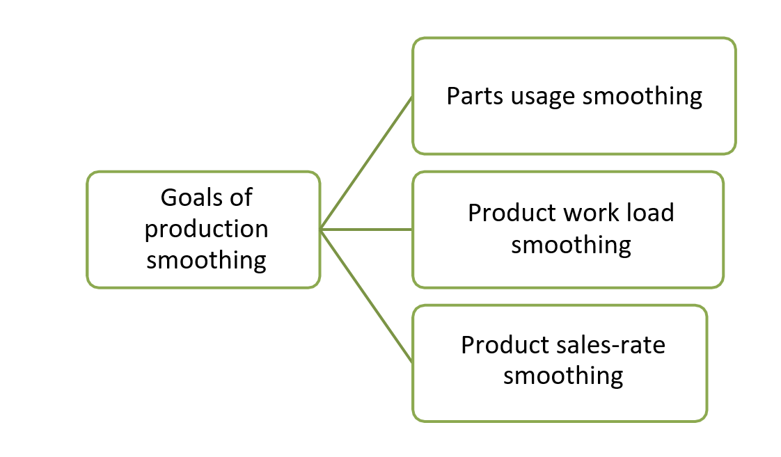
- – Parts usage smoothing(most important goal)
- • Minimize variance in the consumption of parts and/or materials constituting the final products.
- – Product workload smoothing
- • Balancing varied assembly times for continuous flow so that the assembly line does not stop due to the long cycle time processes
- – Product sales-rate smoothing
- • To produce goods with respect to takt tine
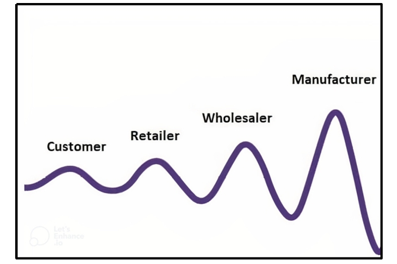
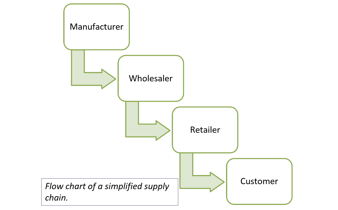
Minimizing Bullwhip effect using Production Smoothing:
- – The Bullwhip effect in supply chain management refers to a situation where even small changes in customer demand can lead to significant
- – To minimize these variations and ensure smoother production production smoothing is done.
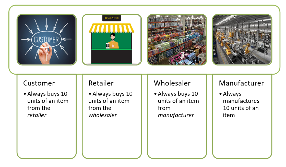
Bullwhip Effect – Case Study:
- – For e.g. Below is an ideal situation where demand always remains constant
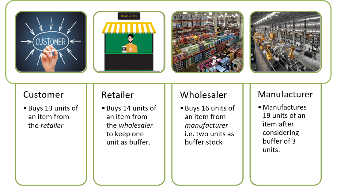
Bullwhip Effect – Case – 1:
- – For e.g. in real-life situations, the demand might vary from let us say 8 to 13 units. Suppose the demand increased to 13 units.
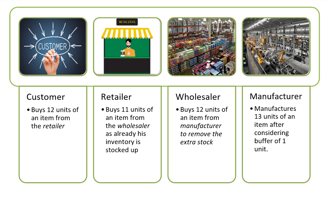
Bullwhip Effect – Case – 2:
- – Now suppose the demand decreased to 12 units.
Bullwhip Effect – Solution:
- – Even with just a 1-unit change in demand, the manufacturer experienced a 6-unit variation in production. Increasing capacity by purchasing new machines would have posed challenges.
- – Here is the solution to overcome the “Bullwhip effect.”
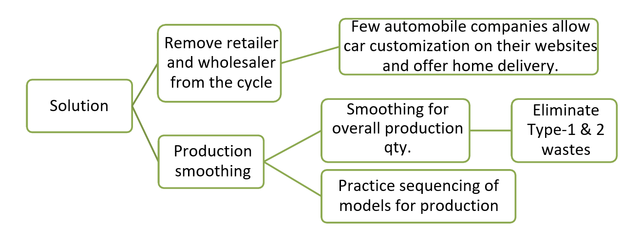
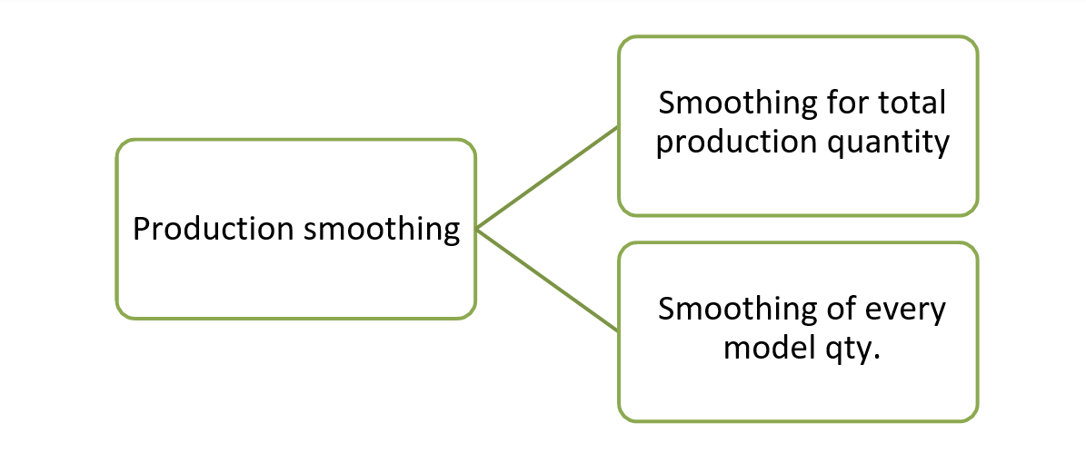
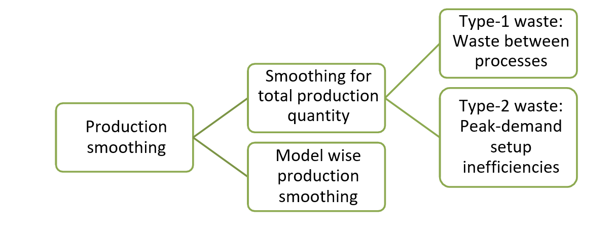
Types of Production Smoothing:
- – One type of production smoothing is to smoothen the production for total quantity. There are two types of waste that need to be eliminated in this type as mentioned below. (Yasuhiro, 4h Edition)
- – Another type is sequencing models for production smoothing.\
Type-1 Waste – Example:
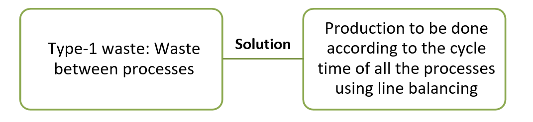
- – Problem statement- Manufacturing has to be done as per takt time = 39 secs. Every workstation exceeds the cycle time of 39 seconds. (A.F.H Fansuri et al 2018)
- – As of now all the processes have a cycle time of more than 39 seconds. Thus, line balancing must be done.
- – Using Ranked Positional Weight method line balancing was done.
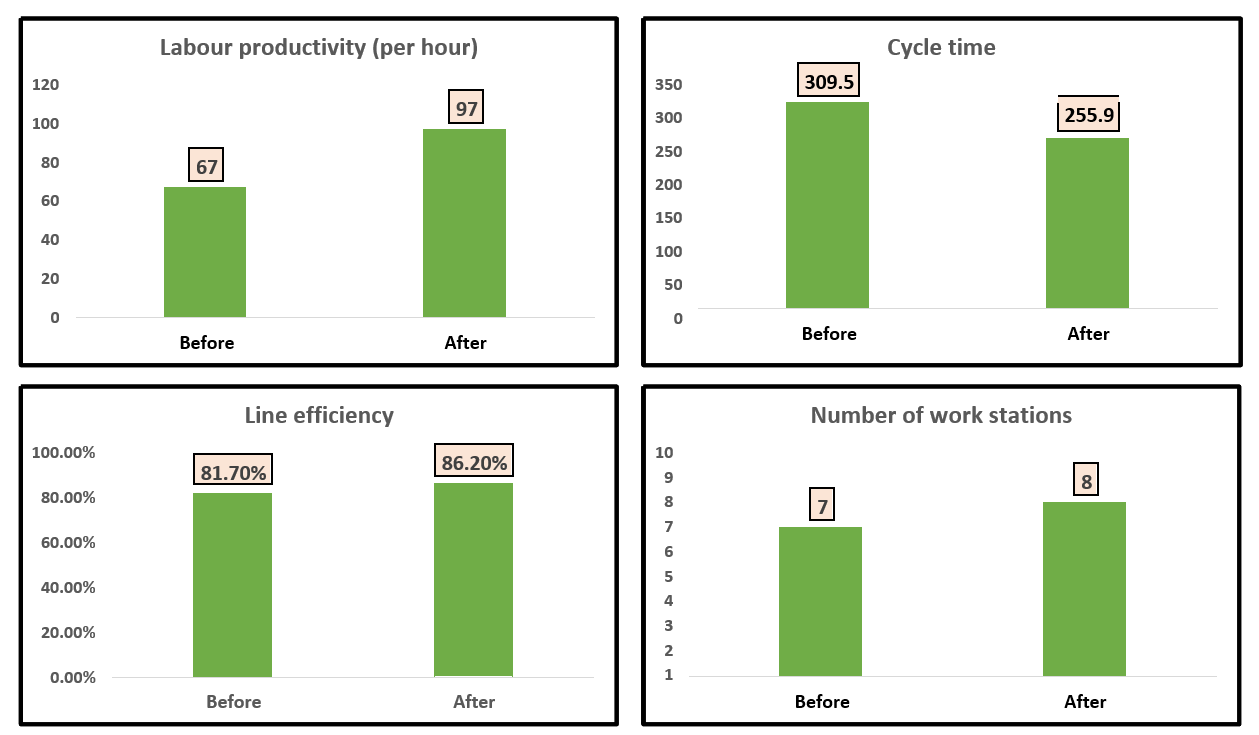
Type-1 Waste Example-Results:
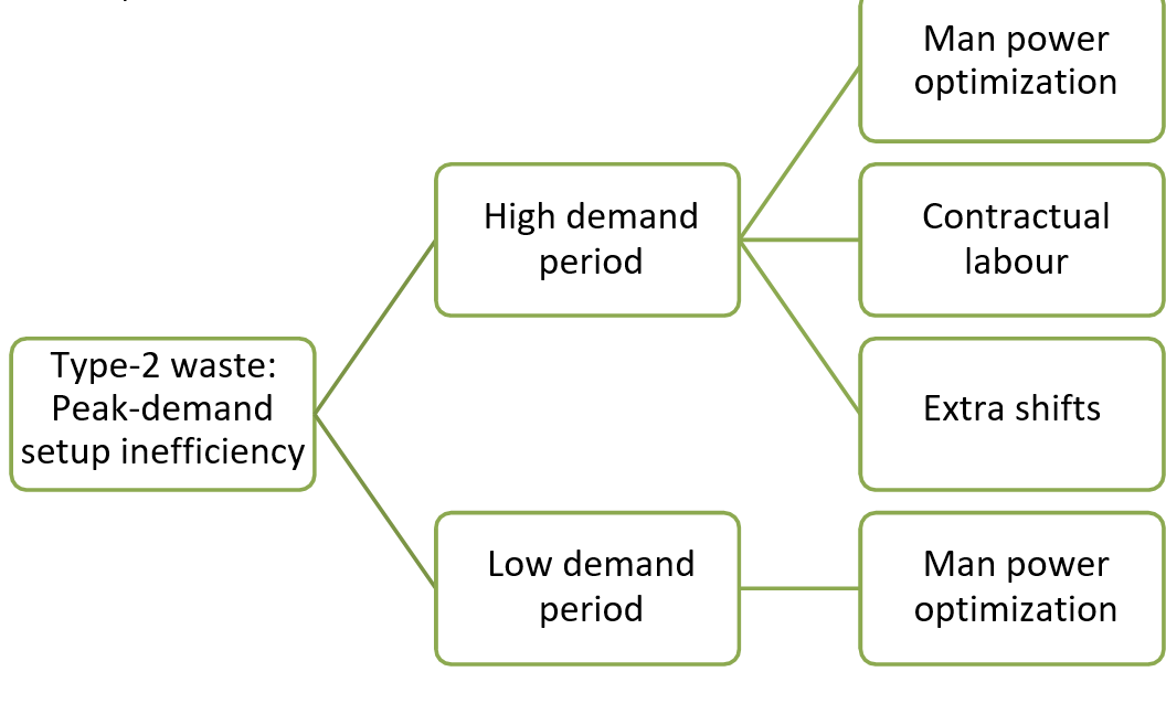
Type-2 Waste:
- – Type-2 waste can be eliminated using the below concepts:(Yasuhiro, 4h Edition)
Model-wise production smoothing-significance:
- – Focusing on a single body type for the entire day results in a substantially larger quantity of finished parts—approximately three to four times more than what is produced with smoothed production. (Yasuhiro, 4th edition)
- – For example, a final assembly line that produces sedans one day, hard tops the next and vans the day after that. A preceding process of making the parts for sedans would have work to do one day, but not again for two days. It would be true for the lines dedicated to vans and hardtops. (Yasuhiro, 4th edition)
- Analyzing the automobile industry, (Swaminathan et. al., 2007) argues that companies can no longer stay profitable by producing large volumes of standardized products.

- (Swaminathan et. al., 2007) states that changes in energy prices and trade structures, internationalization of markets, and increased consumer sophistication are sources for increasing product variety.
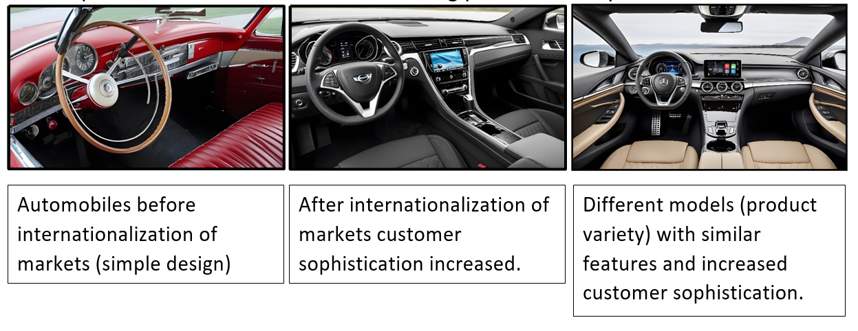
- – Average annual sales per passenger-car model dropped by 34 percent in the United States from 1973 to 1989, while the model count increased from 84 to 142 during this period (Swaminathan et. al., 2007)
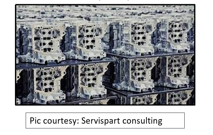
- – Keeping sufficient inventory for a large number of variants can require too much space near the final assembly line. (Swaminathan et. al., 2007)
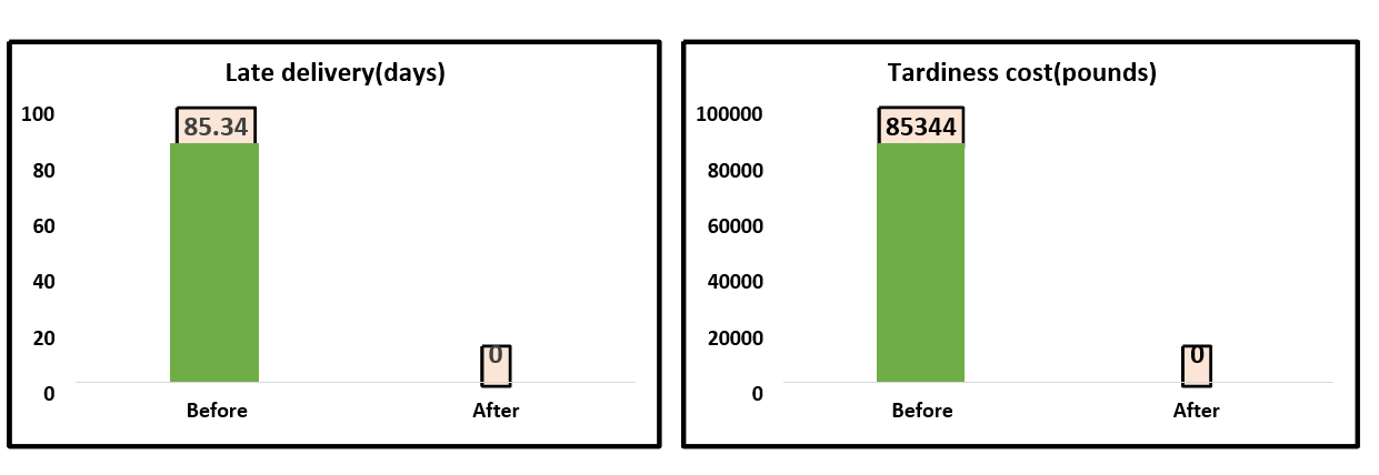
Model-wise production smoothing example:
- – Problem statement- A company was suffering from late time deliveries. To be exact it was 85.34 days. The tardiness cost was 85,344 pounds. Genetic Algorithm was applied for sequencing and below are the results obtained. (P. Pongcharoen et al., 2002)
References:
- – Yasuhiro M. (4h Edition). Toyota Production System. RC Press.
- – A.F.H Fansuri et al 2018 IOP Conf. Ser.: Mater. Sci. Eng. 409 012015
- – Swaminathan and Nitsch: Managing Product Variety in Automobile Assembly
- – M.T. Çelik and S. Arslankaya, Solution of the assembly line balancing problem using the rank positional weight method and Kilbridge and
Wester heuristics method: An application in the cable industry, Journal of Engineering Research, https://doi.org/10.1016/j.jer.2023.100082
- – P. Pongcharoena, C. Hicksa, P.M. Braidena, D.J. Stewardsonb: Determining optimum Genetic Algorithm parameters for scheduling the manufacturing and assembly of complex products.
- – www.servispart.co.uk
- – www.wepik.com
Subscribe
Login
0 Comments